Table of Contents
- 1. Introduction to Autograd
- 2. Back-propagation
- Introduction to Autograd
Autograd is necessary for back-propagation and in Pytorch by making autograd makes back-propagation much easier. There are back-propagation and forward-propagation in neural network.
- Back-propagation
- Let’s say we have a simple neural network where we have only one neuron z, one input data which x, and x is a width of W and bias form of b. In this neuron, we have data in the form of z=W*x + b, so it is a straight linear equation as you can see in figure 1. Then pass that equation through an excitation state where we fit the value of z in the sigmoid function and we get the value of ŷ that is the predicted value for y. This process happens in forwarding pass, all this computation is shown in figure 1 which gives us an image of a graph. This the model of the computation graph.
- Back-propagation

Figure 1 : Computation graph
After we compute ŷ we have to calculate Loss. The loss function can be of any form, here we are taking main square which is basically the mean of actual y minus ŷand its square. In figure 2 as you can see we haven’t shown the mean, it is just the square of the difference since we only have one value. But in real scenario you have to take the mean of all the samples. Once we have the loss function we are ready to calculate the back propagation of the neural network.
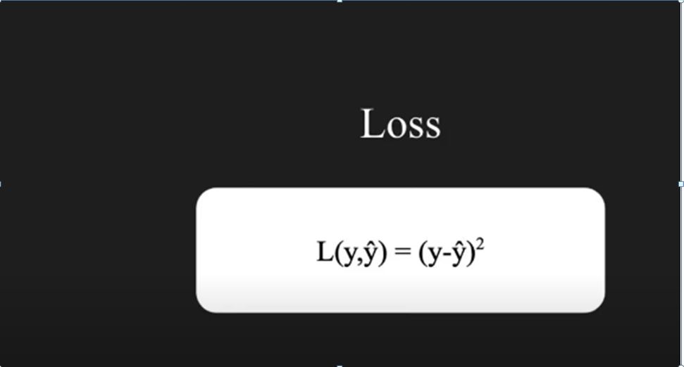
Figure 2: Loss function calculation
Now we will show what happens in back propagation stage, as you can see, we calculate the gradient of each step as you can see in figure 3.
- First we will calculate the partial differentiation of L with respect to ŷ.
- Then we calculate the partial differentiation of ŷ with respect to z.
- Then we calculate the partial differentiation of z with respect to W.
- The main reason to do the above mentioned calculation is because we need the partial differentiation of Loss with
respect to W, so that we can update on the next stage with our learning rate by the chain rule of partial differentiation, we can show that (δL / δW) = (δL / δŷ) * (δŷ / δz) * (δz / δW) as shown in figure 3. In the same way we calculate the partial differentiation with respect to b where we take all the three partial differentiation with respect to L, ŷ and W. Then we calculate the partial differentiation of Loss with respect to b.
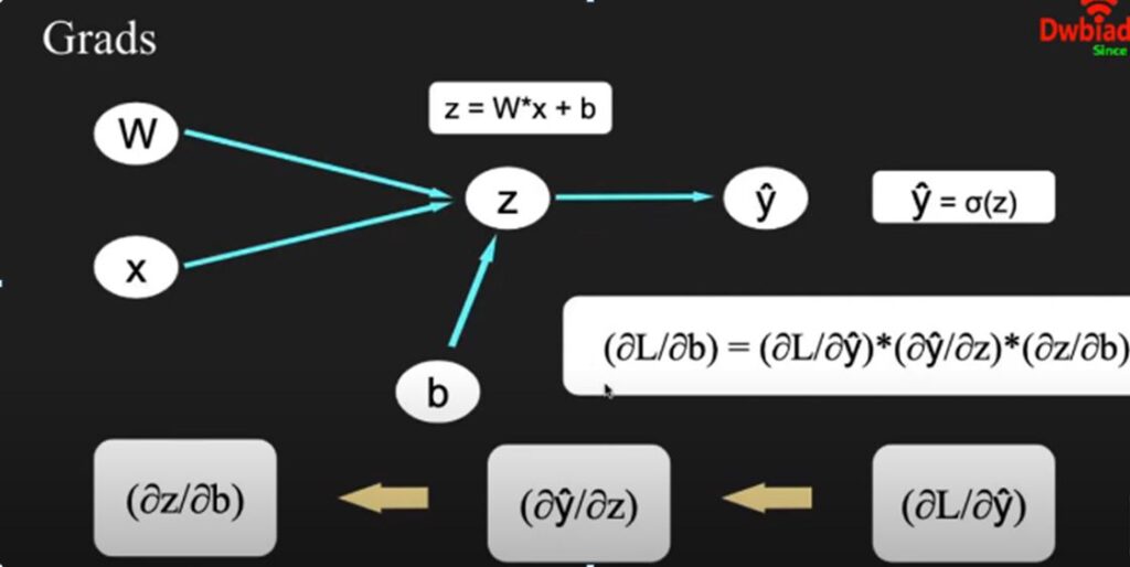
Figure 3: Partial differentiation
By using δL / δW and δL / δb , we can see from the figure 4, this is the heart of the back-propagation stage we have to calculate the W and b with respect to the differentiation we do that using alpha ( α) which is the learning of the formula which you can in the below figure.

Figure 4 :Back-pr0pogation
Lets focus into the coding part:
Pytorch make the calculation easy that you don’t have to add the equations , it will do it for you. Hence Pytorch is so popular, that Pytorch creates the computational graph apart from various other machine learning platforms. Which would create static computation graph, so Pytorch is much better. Lets look into the coding part:
- First we import torch and then we create a variable as you can see the figure 6, which is float 30, we can assign it as x, float 40 in W and float 50 in b.
- Here one thing you might have noticed that we don’t need gradients with respect to x. So In this case requires_grad=False because it differs to we didn’t mention it. In case of W and b we have requires_grad= True in both the cases because we need gradients with respect to W and b. Just to check whether it is a leaf node as shown in the figure 6 we are creating this code b.is_leaf it will be False . But when you check with W and x the value will be True.

Figure 6 : assigning values
Here we keep the calculation simple and we will be calculating the gradient for z =w * x+b . So if z =w * x+b , as you can see from the figure 7. After that we will calculate the and we can see that z is the tensor of value 1250 and it is also a float value. As you want to confirm the value of z, you can use z.is_leaf and the value will be false since W, x and b are the lists and z is the computation based on all these three variables. So z.is_leaf will become a parent now and W,x and b are leaf. But if we calculate ŷ and z.is_leaf, the values will become leaf.

Now lets calculate the gradient:
First to calculate the gradient, we have to write z.backward (), after that it does all the backward calculations for you. When you call backward functions, it calls torch.autograd.backward function which calculates the backward computation and it also creates the computation graph for the differentiation So lets check the value of δz / δw, all you have to do is, write w.grad as we done previously as we stored value 40 in W. After backward calculation value of δz / δw will be stores in W.grad as expected the value is 30 ,and if we check the value of δz / δb , the value will be stores in b.grad and we call it and see the tensor to one as expected as you can see in figure 8.
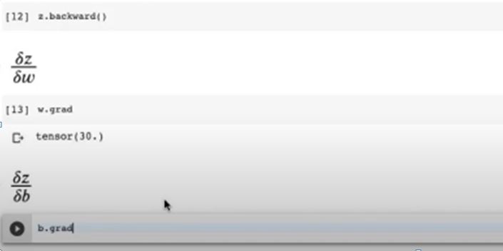
Figure 8: calculating the gradient
So Pytorch makes back-propagation so that you don’t have to all the differentiation and write the functions manually. It all calculates by itself and stores the value properly in grad.
Video Explanation