Recurrent neural network example using data set

Table of Contents

1. Recurrent neural network using surnames dataset
2. Video Explanation ( 2 videos )

Recurrent neural network using surnames dataset

The topic we are going to discuss is the real application of simple RNN model. As we have learned before RNN has a special features from images just like CNN, it is that they learn these features in time, so it is a temple of feature learning.

1. But learning features from the images is not he real application, the recurrent neural network are used to learn text usually and financial data or time series data. The things that change over time, the things the model needs to remember or forget over time, those are the real applications.
2. Now we are going to discuss about the example from the official website called Pytorch. So can download all the datasets from the website of Pytorch. It is the dataset that contains surnames of different countries.
3. So I have uploaded the data.zip folder in the Google colab and when I unzip it , you can see in figure 1, that it has names and inside the names it contains the name of the countries, which are stored as a text file.

So when we open the text file, here are opening Arabic, as you can in figure 2, It has shown all the surnames of those who are from Arabic nationality.

Now we are going to build a model, using RNN that can learn at character level of these surnames of different nationality so that when we predict an unknown surname, it can give us the correct results. So it is called character level text learning. To implement that we have follow certain steps which are:

Firstly we will prepare all the datasets, since it has some surnames of different countries, we are bound to have some peculiar letters as shown in figure 3.

1. As you can see , it has letters with different character, so how can we represent these in English, so for that purpose we have to do some data preparation.
2. First thing to continue is finding all the files that are name.txt.
3. Then we import the unicode data and then we will include all the letters, that are in the ASCII letters and then we will include the character like as shown in figure 4.

If we print the total number of we will see the that we have total of 57 letters as shown in figure 5.

1. Then we will build a model that will learn all the 57 characters and it will correspond to those surnames.
2. There is small function called UnicodToAscii so basically you it an unicode data for example as shown in figure 3, it might be pronounced differently in the country which it belongs to
3. That is the task, we will be converting everything in English so that our model can learn all the letters that are in the ASCII.
4. So firstly we will create a dictionary of all the characters. When we do category line we can see that, our model has learned the surnames from all the text files so Vietnamese has files has certain surnames.
5. That is how our model will be build based on these data.
6. We have all categories which is basically comprised of all the 17 nationality that we have and the read files will read the files and convert everything inside into ASCII. As we have noticed many of the surnames are in the unicode that are not there in English ASCII, so we have to convert all of them and we read all the categories that we have.
7. So we will read the category lines and if we check in n_categories, we can see we have 18 categories.
8. Lets print one of the category. Lets say we want to see the first five surnames in Scottish and as you can see the result in figure 6.

Now lets implement these things in Pytorch.

1. Firstly lets find all the letters in surname, so we convert all the letters to index will create a function that converts all the lines, all the surnames to a tensor, which will convert all the letters to tensors.
2. So as you can see in figure 7, when we convert letter j we will get the following result. When we do line to tensor of John, we can see a big tensor of the size {5, 1, 57}, the 57 is because we have total of 57 characters.

Then lets try with the example of James in the place of John, and as you can see in figure 8, this is how it look like. As we can see that it is the same value as we seen for John. From this we can assume that everything is been converted to this format.

Inside the RNN module, we have the constructor, hidden size, two levels of RNN and in the categorization level we are defining logsoftmax, it is another classification activation function, as shown in figure 9.

1. Finally after the above process we are declaring the forward pass and inithidden basically initialises everything like the hidden layer into with zeros.
2. If we add a letter to tensor and we pass it to our RNN model we get an output, which is shown in figure 10.

1. As can see in the figure 10, after the LogSoftmax, the number has been changed which means our model works.
2. Now try with the example “Adam”.
3. Then we will check what the exact output it is showing, and as you can see in figure 11, the output is going to look like as follows

1. Now we will run our model and create some interesting results.
2. Now we will train our model to learn character by character, so that our model can learn how to construct a surname and tag them according to their classifies nationality.
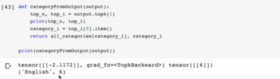
3. So do that we are defining one function as you can see in figure 12. This is called category of output. In this we are inserting that comes from the previous layer that is line to Tensor or letter to Tensor that converts every letter and surnames into tensors, so when we insert our output or tensor converted  surnames into CategoryFromOutput function, it takes the top probability as shown in figure 12, for the category it belongs to according to the model and it prints it out and in the figure 12, you can see the result, which shows you the score of -0.6591 and it belongs to the category Korean and it also prints the index of that category which is 9.

As we recall that there were 18 categories, so maybe in this case it might be confused about the category , as we can see this time it predicted correctly as shown in figure 13, it predicted English.

1. When your model runs many iterations , your model will learn everything eventually.
2. So here we are going to build a SGD model were our model will pick up any random surnames and update our widths and biases.
3. To implement that we are creating Random training example that picks up any random surname from the dataset and train our model. As you can see in figure 14, as we can see it look nationality English and the surname is Burch , then it took the nationality Japanese and it took the surname as Ichigawa.

1. As you can see we are taking our loss function as NLLLoss (), it is a very good loss function when we are implementing Logsoftmax, you might remember from the previous content and it also helpful for the classification task.
2. The learning rate has been set to 0.005 and remember don’t make the value too small otherwise the model won’t run and don’t make it bigger value, other it will explode or vanish.
3. As you can in figure 15, the first train is, and then we initialise all the hidden layer and then we call nn.zero_grad (), which helps in initialising all th gradients after the back propagation.
4. Then we generate the output from the hidden layer that is one RNN module and the output from that RNN module and that will create the input for the next RNN and like that we create a for loop, which actually helps us inserting the output from that hidden layer.
5. We train all the RNN modules, and we train it until we get the input.
6. After that we calculate loss and we calculate loss.backward().
7. As you can notice that we haven’t mentioned any optimiser function that is because we are doing everything manually.
8. After each iteration, as we are picking the values randomly, as you take much bigger value, your model will learn more. So it will print after every 10,000 iteration. So lets our module.
9. So as you can see in figure 15, it has taken random surnames from different datasets and it did it for 1000 iterations.
10. As you notice in the figure that our loss function is being fluctuating a lot.

1. In this case you have to remember that we are creating a structure of the training dataset or the training model that resembles the SGD where it takes one example and takes the model.
2. As we have learned in the previous content, the SGD fluctuates a lot and we haven’t mentioned any optimizer function in any our model, it is basically the batch gradient descent model or we can call it SGD.
3. So here the optimizer in this case is SGD, but we don’t have to worry about the fluctuation in the loss values, it is a bit of technicality.
4. In the training model , we can see that we are printing after every 10,000 steps, so we can see in figure 16, many of the nationality and the surnames has been correctly categorised and, some are incorrect.

1. It is just normal, that when it categorise correctly and some incorrect.
2. So lets continue the evaluation and prediction. So in the evaluation step we initialise all the hidden layers and we generated the outputs and the hidden outputs from each coordinate modules.
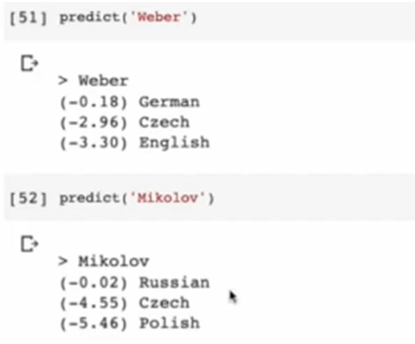
3. In the predict function we will give the input as surnames and we generate three predictions and then we call, torch.no_grad because we don’t want any gradients at that level and then call the evaluate function that we created previously. So in evaluate function we pass a argument line to tensor so it will convert the input surnames to tensor. Then it will evaluate as it it will pass it through all the layers and it will generate the prediction and we are printing the top three predictions as you can see the figure 17.

In the predict function , you can predict any surname you want, as you can see in figure 18, we have taken the example of Rodriguez.

1. As you can see in the figure , the “i” of the Rodriguez is basically not i, but we are converting it into Unicode to ASCII.
2. For more example you can see the figure 19.

So we can see that our model has learned letter by letter or character by character, the surnames and the nationality it belongs to, you can try with new surnames and check whether your model is giving proper input or not.

Video Explanation-part-1

Video Explanation-part-2