Implementing Long Short Term Memory

Table of Contents

1. Implementing Long Short Term Memory
2. Video Explanation

Implementing Long Short Term Memory

1. LSTM is a variant of a recurrent neural networks.
2. Recurrent neural network learns feature from an in-time dataset, that is called temporal future learning. But connecting various neural networks in a series and feeding each of the input data is inefficient, instead, we can modify our structure and we can have better results.
3. One of the biggest drawbacks of the recurrent neural network is vanishing and exploring gradients, that takes place during back propagation over time.
4. The series of a neural network can be very huge and we have to do the back propagation over-time, we have to back-propagate each of the neural networks and when to reach by the last timestamp to the first time stamp in time, the gradients might tend to vanish or explode that is beyond the calculation limit of a computer.
5. Also, the back-propagation over time is a costly process that takes lots of computation which are very complicated.
6. To reduce this computational overhead or remove this problem of exploding and vanishing gradient, LSTM, that is Long Short Term Memory was introduced.
7. In a neural network, tanh function is a very powerful function and tanh activation function has a range from negative one (-1) to positive one (+1).
8. The zero to the negative part of tanh function is used in LSTM or recurrent neural network to forget the memory and the positive half of the tanh function is used to retain a memory and like this way, the neural network decides which data to remember and which data to forget.

Lets begin with the coding part of LSTM:

Firstly we have to import torch, torch.nn, torchvision, torchvision.transforms, torchvision.dataset and importing MNIST, as shown in figure 1

1. In the figure 2, we can see the structure of LSTM model and representation of each symbols in the structure. It shows one cell of a LSTM.
2. Then we call CUDA and then we download the datasets required.
3. As you can see the number of class is 10 , batch size is 100, here we are running two epochs, the learning rate is 0.01.
4. Then we load the train loader and test loader.
5. In the RNN module, in the init function we are calling the input size, hidden size, number of layers and number of classes.
6. We define the hidden size, number of layers and number of classes.
7. Here instead of nn.RNN, we are calling nn.LSTM and this will take care of everything being stored.
8. Make the batch_first =True.
9. In this case, you don’t have to add the non-linearity because it will automatically take care of the sigmoid and tanh activation functions.
10. In the forward pass, we include the input from the previous block for the zeroth instance that is the bunch of zeros and we also have to include C0 is the memory from the previous block, sp now we have two parameters, one is output from the previous block and the other one is memory from the previous block. From that we will get the output from the current block and have a memory from the current block because we don’t want to retain 100 percent of our output.
11. Here we want either partial or sometimes full depending upon the context and finally we print our output.
12. Here the sequence length is 28, number of layers is 2, hidden size is 128 and input size is 28.
13. These goes to the RNN module. Then we instantiate our RNN model.
14. The loss function is CrossEntropyloss.
15. The optimizer is ADAM, and you can change it to RMSProp, so it will perform well.
16. In figure 3, we have total number of steps is equal to length of the train loader, which is basically 600. Then we run the loop of two epochs and each one of them will load the input data. Then we took images and then labels has been taken.

In the forward pass, we predicted the output from the model and then we calculated our loss function and then we did the optimizer.zero_grad, which removes all the gradients and then we calculated the backward propagation over loss and finally optimizer.step updates the weights and biases as you can see in figure 4

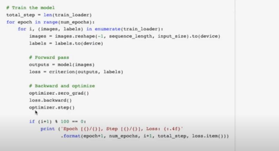
1. Always to remember, all these process is being done under Celestium modules, so this is back-propagation over time.
2. Finally the model is ready after the training and the final loss is 0.2852 and it gives the accuracy of 97.43 percent on 10,000 test images, which is really high.

Video Explanation